utils

Lots of helpful utilities for working with models.

bpreveal.utils.loadModel(modelFname)

Load up a BPReveal model.

Note

Sets bpreveal.internal.constants.GLOBAL_TENSORFLOW_LOADED.

Parameters:

modelFname (str) – The name of the model that Keras saved earlier, either a directory ending in .model for models trained before BPReveal 5.0.0, or a file ending in .keras for models trained with BPReveal 5.0.0 or later.

Returns:

A Keras Model object.

For pre-5.0.0 models, the returned model does NOT support additional training, since it uses a dummy loss. New-style models remember their losses and so you can continue to train them if you like.

Example:

from bpreveal.utils import loadModel
m = loadModel("path/to/model")
preds = m.predict(myOneHotSequences)

bpreveal.utils.setMemoryGrowth()

Turn on the tensorflow option to grow memory usage as needed.

Note

Sets bpreveal.internal.constants.GLOBAL_TENSORFLOW_LOADED.

All of the main programs in BPReveal do this, so that you can use your GPU for other stuff as you work with models.

Return type:

None

bpreveal.utils.loadPisa(fname)

Load up a PISA file, shear it, and crop it to a standard array.

Parameters:

fname (str) – The name of the hdf5-format file on disk, containing your PISA data.

Returns:

An array of shape (num-samples, num-samples) containing the sheared PISA data.

Return type:

ndarray[tuple[int, …], dtype[float16]]

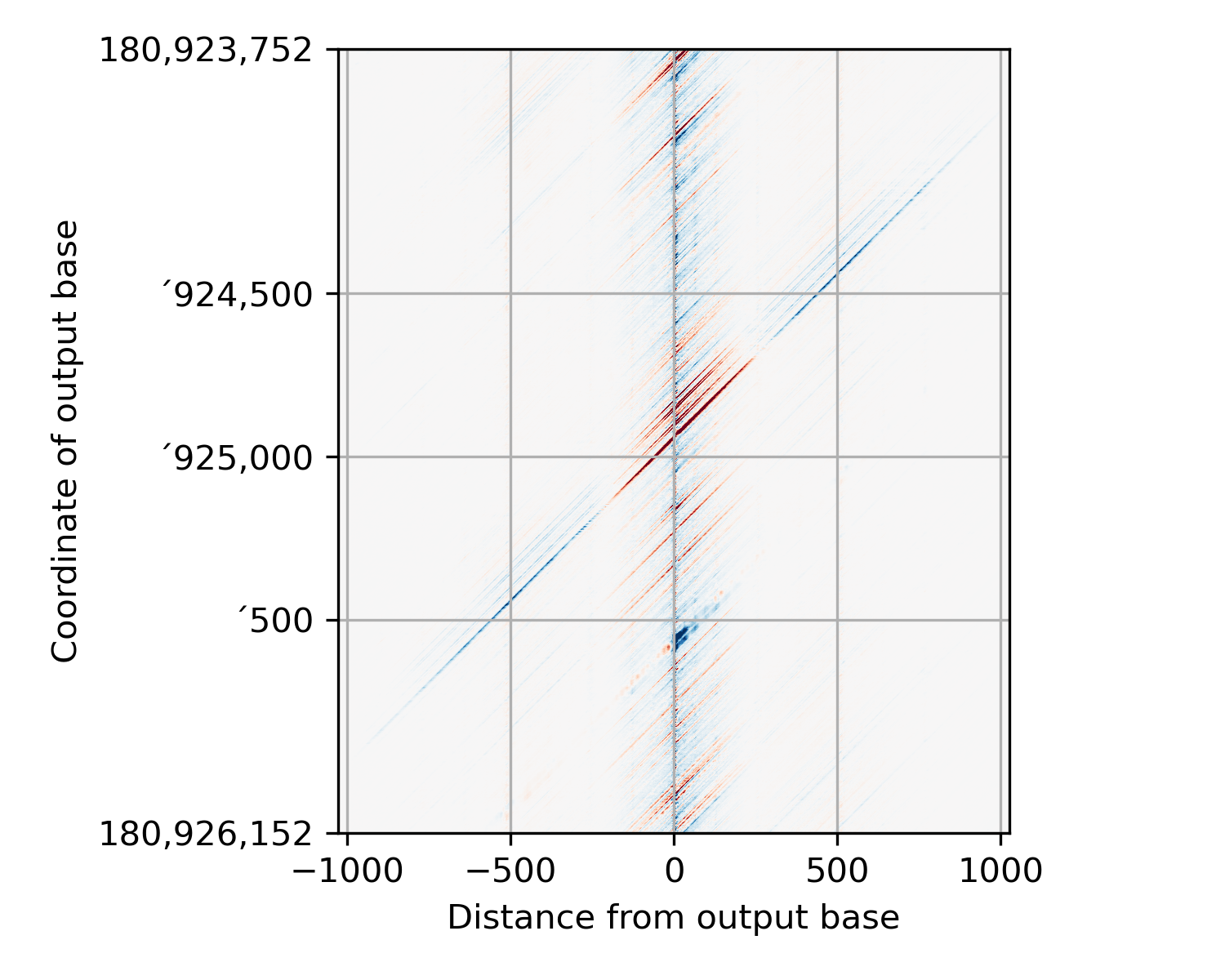
This is probably best demonstrated with an image or two. Here’s how PISA data are stored in the hdf5 file:

This function first shears the PISA data into a more normal form:

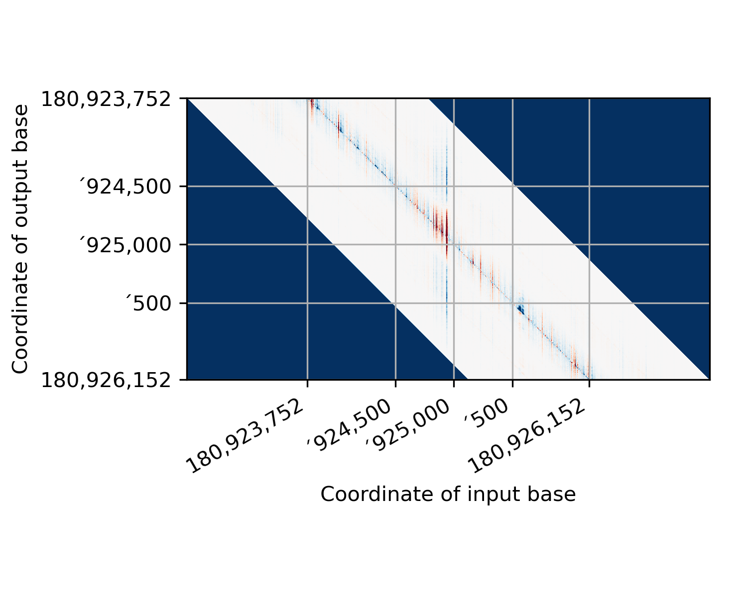
(In this figure, I’ve colored pixels where we didn’t have any starting data dark blue so that they stand out.) There is a lot of wasted space in this image. So we crop it by deleting receptiveField // 2 pixels from each side: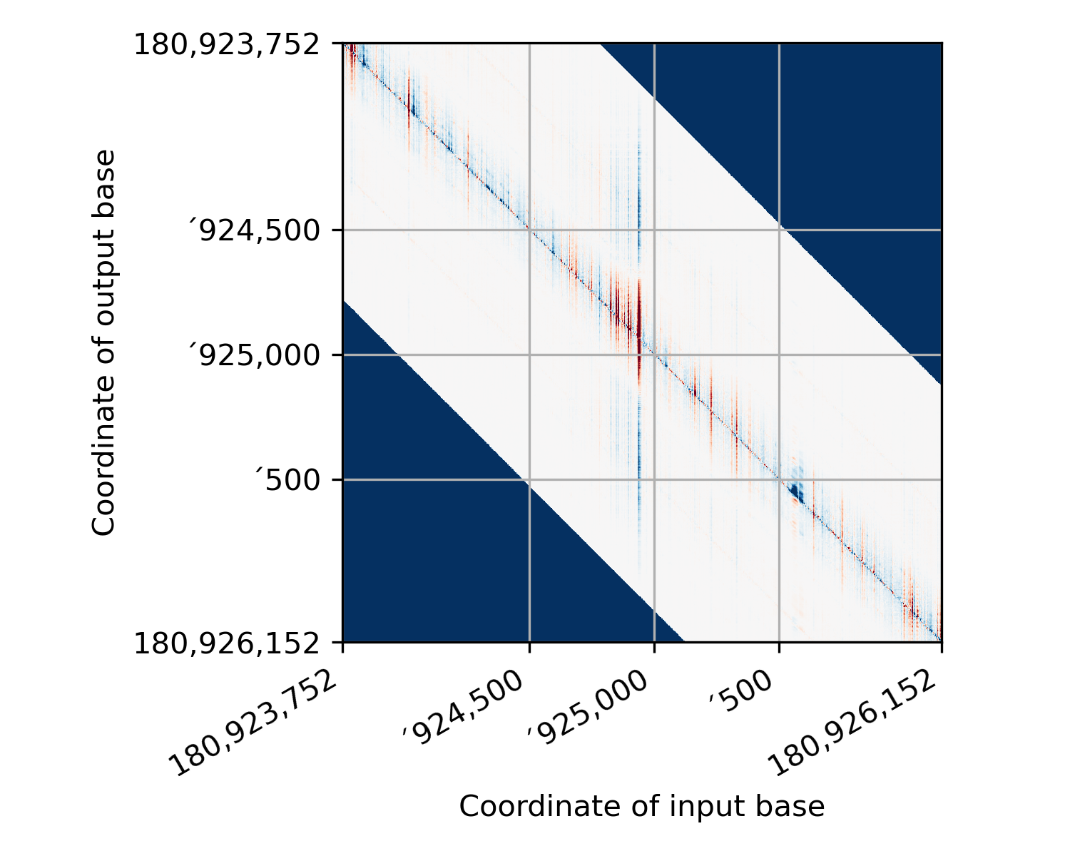

This is the output of this function. (except that I have added in the dark blue patches where there was no data before shearing - the actual return from this function just contains zeros in those regions.) Now, in preparing your regions to run PISA, you need to be pretty careful so that the coordinate you think you are explaining is actually the one that the PISA starts with! Here’s a representation of where each base in the sheared image comes from, relative to the actual model input:

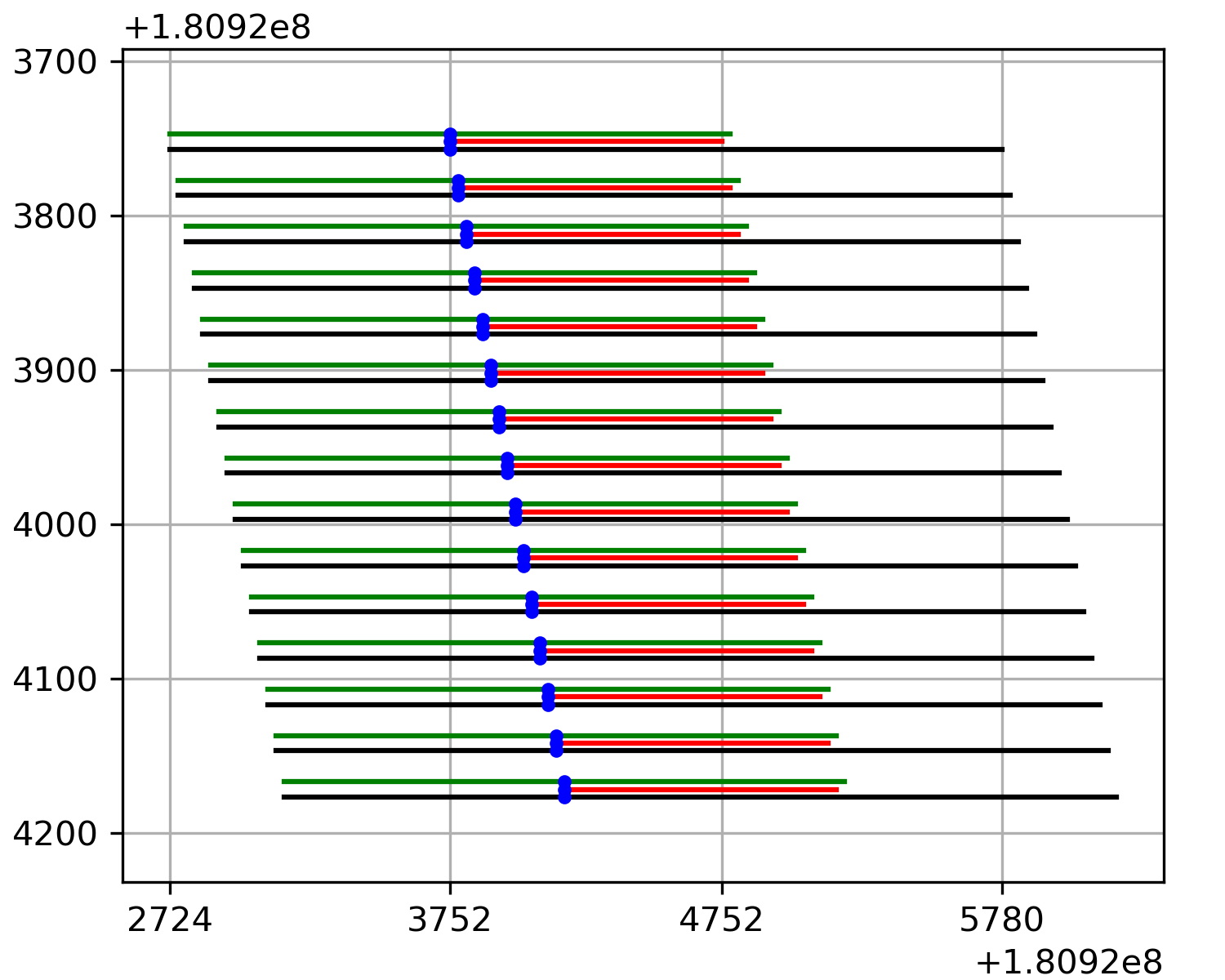
In this figure, the input to the model is shown in black, the model’s output is shown in red, and output being explained is shown as a blue dot. The green line shows the receptive field of the model centered around the output base (This is where we have data in the PISA plot). I’ve put some helpful marks on the x-axis that line up with the topmost PISA row. If you supply a bed file to the PISA interpretation script, then it will provide PISA values where each base in the window is an output from the model. In other words, the bed file for these data would have started at position ‘3752. This keeps life easy, and it also means that when you use this function, the array that gets loaded corresponds exactly to the bed region you used.

If, however, you use a fasta-format input, things get hairy. The fasta-format input must contain enough bases to fill the entire model’s input (i.e., the black lines in this figure), and so it will include bases to the left of the output being explained. The number of padding bases will be receptiveField // 2. In this case, my receptive field is 2057, and so there are 1028 extra bases on the left of the blue output being explained.

Each entry in a fasta file could in principle be a completely different sequence. However, to make a comprehensible PISA plot, the sequences will typically all be drawn from the same region but offset by one each time. In other words, the lines in the fasta file would be the black lines in this figure.

This line diagram represents the uncropped data. The matrix returned from this function would start at position ‘3752 and end at 3752 + numEntries.

bpreveal.utils.limitMemoryUsage(fraction, offset)

Limit tensorflow to use only the given fraction of memory.

Note

Sets bpreveal.internal.constants.GLOBAL_TENSORFLOW_LOADED.

This will allocate total-memory * fraction - offset Why use this? Well, for running multiple processes on the same GPU, you don’t want to have them both allocating all the memory. So if you had two processes, you’d do something like:

def child1():
    utils.limitMemoryUsage(0.5, 1024)
    # Load model, do stuff.

def child2():
    utils.limitMemoryUsage(0.5, 1024)
    # Load model, do stuff.

p1 = multiprocessing.Process(target=child1); p1.start()
p2 = multiprocessing.Process(target=child2); p2.start()

And now each process will use (1024 MB less than) half the total GPU memory.

Parameters:

• fraction (float) – How much of the memory on the GPU can I have?

• offset (float) – How much memory (in MB) should be reserved when I carve out my fraction?

Returns:

The memory (in MB) reserved.

Return type:

float

bpreveal.utils.loadChromSizes(*, chromSizesFname=None, genomeFname=None, bwHeader=None, bw=None, fasta=None)

Read in a chrom sizes file and return a dictionary mapping chromosome name → size.

Exactly one of the parameters may be specified, all others must be None.

Parameters:

• chromSizesFname (str | None) – The name of a chrom.sizes file on disk.

• genomeFname (str | None) – The name of a genome fasta file on disk.

• bwHeader (dict[str, int] | None) – A dictionary loaded from a bigwig. (Using this makes this function an identity function.)

• bw (bigWigFile | None) – An opened bigwig file.

• fasta (FastaFile | None) – An opened genome fasta.

Returns:

{“chr1”: 1234567, “chr2”: 43212567, …}

Return type:

dict[str, int]

Example:

from bpreveal.utils import loadChromSizes, blankChromosomeArrays, writeBigwig
import pysam
genome = pysam.FastaFile("path/to/genome.fa")
chromSizeDict = loadChromSizes(fasta=genome)
chromArs = blankChromosomeArrays(chromSizes=chromSizeDict, numTracks=1)
myRegionDats = ...  # Some function that returns tuples of (chrom, start, end, data)
for rChrom, rStart, rEnd, rValues in myRegionDats:
    chromArs[rChrom][rStart:rEnd] = rValues
writeBigwig(bwFname="path/to/output.bw", chromArs)

bpreveal.utils.blankChromosomeArrays(*, genomeFname=None, chromSizesFname=None, bwHeader=None, chromSizes=None, bw=None, fasta=None, dtype=<class 'numpy.float32'>, numTracks=1)

Get a set of blank numpy arrays that you can use to save genome-wide data.

Exactly one of chromSizesFname, genomeFname, bwHeader, chromSizes, bw, or fasta may be specified, all other parameters must be None.

Parameters:

• chromSizesFname (str | None) – The name of a chrom.sizes file on disk.

• genomeFname (str | None) – The name of a genome fasta file on disk.

• bwHeader (dict[str, int] | None) – A dictionary loaded from a bigwig.

• chromSizes (dict[str, int] | None) – A dictionary mapping chromosome name to length.

• bw (bigWigFile | None) – An opened bigwig file.

• fasta (FastaFile | None) – An opened genome fasta.

• dtype (type) – The type of the arrays that will be returned.

• numTracks (int) – How many tracks of data do you have?

Returns:

A dict mapping chromosome name to a numpy array.

Return type:

dict[str, ndarray]

The returned dict will have an element for every chromosome in the input. The shape of each element of the dictionary will be (chromosome-length, numTracks).

See loadChromSizes for an example.

bpreveal.utils.writeBigwig(bwFname, chromDict=None, regionList=None, regionData=None, chromSizes=None)

Write a bigwig file given some region data.

You must specify either:

• chromDict,

  in which case regionList, chromSizes and regionData must be None, or

• regionList, chromSizes, and regionData,

  in which case chromDict must be None.

Parameters:

• bwFname (str) – The name of the bigwig file to write.

• chromDict (dict[str, ndarray] | None) – A dict mapping chromosome names to the data for that chromosome. The data should have shape (chromosome-length,).

• regionList (list[tuple[str, int, int]] | None) – A list of (chrom, start, end) tuples giving the locations where the data should be saved.

• regionData (Any) – An iterable with the same length as regionList. The ith element of regionData will be written to the ith location in regionList.

• chromSizes (dict[str, int] | None) – A dict mapping chromosome name → chromosome size.

Return type:

None

See loadChromSizes for an example.

bpreveal.utils.oneHotEncode(sequence, allowN=False, alphabet='ACGT')

Convert the string sequence into a one-hot encoded numpy array.

Parameters:

• sequence (str) – A DNA sequence to encode. May contain uppercase and lowercase letters.

• allowN (bool) – If False (the default), raise an AssertionError if the sequence contains letters other than ACGTacgt. If True, any other characters will be encoded as [0, 0, 0, 0].

• alphabet (str) – The order of the bases in the output array.

Returns:

An array with shape (len(sequence), NUM_BASES).

Return type:

`` ONEHOT_AR_T ``

The columns are, in order, A, C, G, and T. The mapping is as follows:

A or a → [1, 0, 0, 0]
C or c → [0, 1, 0, 0]
G or g → [0, 0, 1, 0]
T or t → [0, 0, 0, 1]
Other  → [0, 0, 0, 0]

A convenient property of this mapping is that calculating a reverse-complement sequence is trivial:

seq = "AAGAGGCT"
ohe = oneHotEncode(seq)
revcompOhe = np.flip(ohe)
revcompSeq = oneHotDecode(revcompOhe)
# revcompSeq is now "AGCCTCTT"

Example:

from bpreveal.utils import oneHotEncode, oneHotDecode
seq = "ACGTTT"
x = oneHotEncode(seq)
print(x)
# [[1 0 0 0]
#  [0 1 0 0]
#  [0 0 1 0]
#  [0 0 0 1]
#  [0 0 0 1]
#  [0 0 0 1]]
y = oneHotDecode(x)
print(y)
# ACGTTT

bpreveal.utils.oneHotDecode(oneHotSequence, alphabet='ACGT')

Take a one-hot encoded sequence and turn it back into a string.

Parameters:

• oneHotSequence (ndarray) – An array of shape (n, NUM_BASES). It may have any type that can be converted into a uint8.

• alphabet (str) – The order in which the bases are encoded.

Return type:

str

Given an array representing a one-hot encoded sequence, convert it back to a string. The input shall have shape (sequenceLength, NUM_BASES), and the output will be a Python string. The decoding is performed based on the following mapping:

[1, 0, 0, 0] → A
[0, 1, 0, 0] → C
[0, 0, 1, 0] → G
[0, 0, 0, 1] → T
[0, 0, 0, 0] → N

See oneHotEncode for an example.

bpreveal.utils.logitsToProfile(logitsAcrossSingleRegion, logCountsAcrossSingleRegion)

Take logits and logcounts and turn it into a profile.

Parameters:

• logitsAcrossSingleRegion (`` LOGIT_AR_T ``) – An array of shape (output-length * num-tasks)

• logCountsAcrossSingleRegion (`` LOGCOUNT_T ``) – A single floating-point number

Returns:

An array of shape (output-length * num-tasks), giving the profile predictions.

Return type:

`` PRED_AR_T ``

Example:

from bpreveal.utils import loadModel, oneHotEncode, logitsToProfile
import pysam
import numpy as np
genome = pysam.FastaFile("/scratch/genomes/sacCer3.fa")
seq = genome.fetch("chrII", 429454, 432546)
oneHotSeq = oneHotEncode(seq)
print(oneHotSeq.shape)
model = loadModel("/scratch/mnase.model")
preds = model.predict(np.array([oneHotSeq]))
print(preds[0].shape)
# > (1, 1000, 2)
# because there was one input sequence, the output-length is 1000 and
# there are two tasks in this head.
print(preds[1].shape)
# > (1, 1)
# because there is one input sequence and there's just one logcounts value
# for each region.
# Note that if the model had two heads, preds[1] would be the logits from the
# second head and preds[2] and preds[3] would be the logcounts from head 1 and
# head 2, respectively.
profiles = logitsToProfile(preds[0][0], preds[1][0])
print(profiles.shape)
# > (1000, 2)
# Because we have an output length of 1000 and two tasks.
# These are now the predicted coverage, in read-space.

bpreveal.utils.easyPredict(sequences, modelFname, quiet=False)

Make predictions with your model.

Parameters:

• sequences (Iterable[str] | str) – The DNA sequence(s) that you want to predict on.

• modelFname (str) – The name of the Keras model to use.

• quiet (bool) – If True, all stderr spew from tensorflow is deleted. Set to True for interactive use, but set to False if you’re getting errors, since they’ll be deleted otherwise and make debugging a nightmare.

Returns:

An array of profiles or a single profile, depending on sequences

Return type:

list[list[ :py:data:`PRED_AR_T<bpreveal.internal.constants.PRED_AR_T>` ]] or list[ :py:data:`PRED_AR_T<bpreveal.internal.constants.PRED_AR_T>` ]

Spawns a separate process to make a single batch of predictions, then shuts it down. Why make it complicated? Because it frees the GPU after it’s done so other programs and stuff can use it. If sequences is a single string containing a sequence to predict on, that’s okay, it will be treated as a length-one list of sequences to predict. The sequences string should be at least as long as the input length of your model.

If you passed in an iterable of strings (like a list of strings), the shape of the returned profiles will be (numSequences x numHeads x outputLength x numTasks). Since different heads can have different numbers of tasks, the returned object will be a list (one entry per sequence) of lists (one entry per head) of arrays of shape (outputLength x numTasks). If, instead, you passed in a single string as sequences, it will be (numHeads x outputLength x numTasks). As before, this will be a list (one entry per head) of arrays of shape (outputLength x numTasks)

As a bonus feature, if you pass in a sequence that is longer than your model’s input length, this function will make tiling predictions over as much of the sequence as possible. For example, if my model has an input length of 3 kb and an output of 1 kb, then if I provide an input sequence that is 4 kb long, I will get a 2 kb output prediction.

Example:

from bpreveal.utils import easyPredict
import pysam
genome = pysam.FastaFile("/scratch/genomes/sacCer3.fa")
seq = genome.fetch("chrII", 429454, 432546)
profile = easyPredict([seq], "/scratch/mnase.model")
print(len(profile))
# > 1
# because we ran one sequence.
print(len(profile[0]))
# > 1
# because there is one head in this model.
print(profile[0][0].shape)
# > (1000, 2)
# Because we have an output length of 1000 and two tasks.
# These are now the predicted coverage, in read-space.
singleProfile = easyPredict(seq, "/scratch/mnase.model")
print(singleProfile[0].shape)
# > (1000, 2)
# Note how I only had to index singleProfile once, (to get the first head)
# since I passed in a single string as the sequence.

bpreveal.utils.easyInterpretFlat(sequences, modelFname, heads, headID, taskIDs, numShuffles=20, kmerSize=1, keepHypotheticals=False)

Spin up an entire interpret pipeline just to interpret your sequences.

You should only use this for quick one-off things since it takes a long time to spin up and shut down the interpretation machinery.

Parameters:

• sequences (Iterable[str] | str) – is a list (or technically any Iterable) of strings, and the returned importance scores will be in an order that corresponds to your sequences. You can also provide just one string, in which case the return type will change: The first (length-one) dimension will be stripped.

• modelFname (str) – The name of the BPReveal model on disk.

• heads (int) – The TOTAL number of heads that the model has.

• headID (int) – The index of the head of the model that you want interpreted.

• taskIDs (list[int]) – The list of tasks that should be included in the profile score calculation. For most cases, you’d want a list of all the tasks, like [0,1].

• numShuffles (int) – The number of shuffled sequences that are used to calculate shap values.

• kmerSize (int) – The length of kmers for which the distribution should be preserved during the shuffle. If 1, shuffle each base independently. If 2, preserve the distribution of dimers, etc.

• keepHypotheticals (bool) – Controls whether the output contains hypothetical contribution scores or just the actual ones.

Returns:

A dict containing the importance scores.

Return type:

dict[str,  :py:data:`IMPORTANCE_AR_T<bpreveal.internal.constants.IMPORTANCE_AR_T>`  |  :py:data:`ONEHOT_AR_T<bpreveal.internal.constants.ONEHOT_AR_T>` ]

If you passed in an iterable of strings (like a list), then the output’s first dimension will be the number of sequences and it will depend on keepHypotheticals:

• If keepHypotheticals == True, then it will be structured so:

  {"profile": array of shape (numSequences x inputLength x NUM_BASES),
   "counts": array of shape (numSequences x inputLength x NUM_BASES),
   "sequence": array of shape (numSequences x inputLength x NUM_BASES)}
  

  This dict has the same meaning as shap scores stored in an interpretFlat hdf5.

• If keepHypotheticals == False (the default), then the shap scores will be condensed down to the normal scores that we plot in a genome browser:

  {"profile": array of shape (numSequences x inputLength),
   "counts": array of shape (numSequences x inputLength)}
  

However, if sequences was a string instead of an iterable, then the numSequences dimension will be suppressed:

• For keepHypotheticals == True, you get:

  {"profile": array of shape (inputLength x NUM_BASES),
   "counts": array of shape (inputLength x NUM_BASES),
   "sequence": array of shape (inputLength x NUM_BASES)}
  

• and if keepHypotheticals == False, you get:

  {"profile": array of shape (inputLength,),
   "counts": array of shape (inputLength,)}
  

class bpreveal.utils.BatchPredictor(modelFname, batchSize, start=True, numThreads=0, produceProfiles=False, quiet=False)

A utility class for when you need to make lots of predictions.

Note

Sets bpreveal.internal.constants.GLOBAL_TENSORFLOW_LOADED.

It’s doubly-useful if you are generating sequences dynamically. Here’s how it works. You first create a predictor by calling BatchPredictor(modelName, batchSize). If you’re not sure, a batch size of 64 is probably good.

Now, you submit any sequences you want predicted, using the submit methods.

Once you’ve submitted some or all of your sequences, you can get your results with the getOutput() method.

Note that the getOutput()` method returns *one* result at a time, and you have to call ``getOutput() once for every time you called one of the submit methods.

The typical use case for a batcher streams its input, so you’d normally check to see if there’s output waiting after adding every input:

for query, label in queryGenerator:
    batcher.submitString(query, label)
    while batcher.outputReady():
        # Any time the batcher has results, process them
        # immediately.
        preds, outLabel = batcher.getOutput()
        processPredictions(preds, outLabel)
while not batcher.empty():
    # We've finished adding our queries, now drain out
    # any last results.
    preds, outLabel = batcher.getOutput()
    processPredictions(preds, outLabel)

Using the batcher in this way (checking to see if outputReady() after every query submission) has the benefit of using very little memory. Instead of building a huge array of queries and then predicting them in one go, the batcher analyzes them as you come up with them. This means you can analyze far more sequences than you can store in memory. (But if you have huge numbers of sequences, consider using a ThreadedBatchPredictor since it can do the calculations in parallel and in a separate thread.)

For small numbers of sequences, you can also submit all of them and then get all of the results later:

for i in range(numQueries):

batcher.submitString(queries[i], None)

for _ in range(numQueries):

preds, _ = batcher.getOutput() processPredictions(preds)

In this example, I’m not using the labels, so I just pass in None as the label for each sequence and ignore the labels from getOutput()

You should not, however, demand an output after every submission, since this will use a batch size of one and be painfully slow:

for query, label in queryGenerator:
    batcher.submitString(query, label)
    preds, outLabel = batcher.getOutput()  # WRONG: Runs a whole batch for each query
    processPredictions(preds, outLabel)

Parameters:

• modelFname (str) – The name of the BPReveal model on disk that you want to make predictions from. It’s the same name you give for the model in any of the other BPReveal tools.

• batchSize (int) – is the number of samples that should be run simultaneously through the model.

• start (bool) – Ignored, but present here to give BatchPredictor the same API as ThreadedBatchPredictor. Creating a BatchPredictor loads up the model and sets memory growth right then and there.

• numThreads (int) – Ignored, only present for compatibility with the API for ThreadedBatchPredictor. A (non-threaded)``BachPredictor`` runs its calculations in the main thread and will block when it’s actually doing calculations.

• produceProfiles (bool) – Ignored, only for compatibility with ThreadedBatchPredictor. With a non-threaded BatchPredictor, you can choose to use getOutput() or getOutputProfile() after the prediction has been made.

• quiet (bool) – If True, then all output to stderr will be suppressed in tensorflow-related code. Useful for interactive use.

clear()

Reset the predictor.

If you’ve left your predictor in some weird state, you can reset it by calling clear(). This empties all the queues.

Return type:

None

submitOHE(sequence, label)

Submit a one-hot-encoded sequence.

Parameters:

• sequence (ndarray[tuple[int, ...], dtype[uint8]]) – An (input-length x NUM_BASES) ndarray containing the one-hot encoded sequence to predict.

• label (Any) – Any object; it will be returned with the prediction.

Return type:

None

submitString(sequence, label)

Submit a given sequence for prediction.

Parameters:

• sequence (str) – A string of length input-length

• label (Any) – Any object. Label will be returned to you with the prediction.

Return type:

None

runBatch(maxSamples=None)

Actually run the batch.

Normally, this will be called by the submit functions, and it will also be called if you ask for output and the output queue is empty (assuming there are sequences waiting in the input queue.) In other words, you don’t need to call this function.

Parameters:

maxSamples (int | None) – (Optional) The maximum number of samples to run in this batch. It should probably be a multiple of the batch size.

Return type:

None

outputReady()

Is there any output ready for you?

If output is ready, then calling getOutput() will give a result immediately.

Returns:

True if the batcher is sitting on results, and False otherwise.

Return type:

bool

empty()

Is the batcher totally idle?

If the batcher is not empty, then you can safely call getOutput(), though it may block if it needs to run a calculation.

Returns:

True if there are no predictions at all in the queue.

Return type:

bool

getOutput()

Return one of the predictions made by the model.

This implementation guarantees that predictions will be returned in the same order as they were submitted.

Returns:

A two-tuple.

Return type:

tuple[list[ :py:data:`LOGIT_AR_T<bpreveal.internal.constants.LOGIT_AR_T>` ,  :py:data:`LOGIT_T<bpreveal.internal.constants.LOGIT_T>` ], typing.Any]

• The first element will be a list of length numHeads * 2, representing the output from the model. Since the output of the model will always have a dimension representing the batch size, and this function only returns the result of running a single sequence, the dimension representing the batch size is removed. In other words, running the model on a single example would give a logits output of shape (1 x output-length x num-tasks). But this function will remove that, so you will get an array of shape (output-length x numTasks) As with calling the model directly, the first numHeads elements are the logits arrays, and then come the logcounts for each head. You can pass the logits and logcounts values to utils.logitsToProfile to get your profile.

• The second element will be the label you passed in with the original sequence.

Graphically:

( [<head-1-logits>, <head-2-logits>, ...
   <head-1-logcounts>, <head-2-logcounts>, ...
  ],
  label)

If the batcher doesn’t have any output ready but does have some work in the input queue, then calling this function will block until the calculation is complete. If there is output ready, then this function will not block.

This function will error out if an input sequence was longer than the model’s input length, since there’s no logical way to combine the logits and logcounts in that case. If you want to use longer sequences, you should get outputs with getOutputProfile().

getOutputProfile()

Return one of the predictions made by the model, in profile space.

Whereas getOutput returns the logits and logcounts directly from the model, this function converts those results into a profile. This is necessary if you provide an input sequence that is longer than the model’s input length.

This implementation guarantees that predictions will be returned in the same order as they were submitted.

Returns:

A two-tuple.

Return type:

tuple[list[ :py:data:`PRED_AR_T<bpreveal.internal.constants.PRED_AR_T>` ], typing.Any]

• The first element will be a list of length numHeads, representing the output from the model. Since the output of the model will always have a dimension representing the batch size, and this function only returns the result of running a single sequence, the dimension representing the batch size is removed. In other words, running the model on a single example would give a profile of shape (1 x output-length x num-tasks). But this function will remove that, so you will get an array of shape (output-length x numTasks)

• The second element will be the label you passed in with the original sequence.

Graphically:

( [<head-1-profile>, <head-2-profile>, ...],
  label)

If the batcher doesn’t have any output ready but does have some work in the input queue, then calling this function will block until the calculation is complete. If there is output ready, then this function will not block.

class bpreveal.utils.ThreadedBatchPredictor(modelFname, batchSize, start=False, numThreads=1, produceProfiles=False, quiet=False)

Mirrors the API of BatchPredictor, but predicts in a separate thread.

This can give you a performance boost, and also lets you shut down the predictor thread when you don’t need it (thus freeing the GPU for other things). Supports the with statement to only turn on the batcher when you’re using it, or you can leave it running in the background.

Usage examples:

predictor = utils.ThreadedBatchPredictor(modelFname, 64, start=True)
# Use as you would a normal batchPredictor
# When not needed any more:
predictor.stop()

Alternatively, you can use this as a context manager:

predictor = utils.ThreadedBatchPredictor(modelFname, 64, start=False)

with predictor:
    # use as a normal BatchPredictor.
# On leaving the context, the predictor is shut down.
# But you can spin it up if you need it again:
with predictor:
    # use the predictor some more.

The batcher guarantees that the order in which you get results is the same as the order you submitted them in, even though the internal calculations may happen out-of-order.

Parameters:

• modelFname (str) – The name of the model to use to make predictions.

• batchSize (int) – The number of samples to calculate at once.

• start (bool) – Should the predictor start right away? This should be False if you’re going to use this ThreadedBatchPredictor inside a context manager (i.e., a with statement).

• numThreads (int) – How many predictors should be spawned? I recommend 2 or 3.

• produceProfiles (bool) – If True, then you can call getOutputProfile() If False (the default), then you can only call getProfile(). You have to specify this before starting the batcher because the profile production is done in parallel and so this class needs to know what sort of output you will want so it can have it ready for you when you need it.

• quiet (bool) – If True, redirect all stdout from tensorflow to the trash.

start()

Spin up the batcher thread.

If you submit sequences without starting the batcher, this method will be called automatically (with a warning).

Return type:

None

stop()

Shut down the processor thread.

Return type:

None

clear()

Reset the batcher, emptying any queues and reloading the model.

This also starts the batcher.

Return type:

None

submitOHE(sequence, label)

Submit a one-hot-encoded sequence.

Parameters:

• sequence (ndarray[tuple[int, ...], dtype[uint8]]) – An (input-length x NUM_BASES) ndarray containing the one-hot encoded sequence to predict.

• label (Any) – Any (picklable) object; it will be returned with the prediction.

Return type:

None

submitString(sequence, label)

Submit a given sequence for prediction.

Parameters:

• sequence (str) – A string of length input-length

• label (Any) – Any (picklable) object. Label will be returned to you with the prediction.

Return type:

None

outputReady()

Is there any output ready for you?

If output is ready, then calling getOutput() will give a result immediately.

Returns:

True if the batcher is sitting on results, and False otherwise.

Return type:

bool

empty()

Is the batcher totally idle?

If the batcher is not empty, then you can call getOutput(), though it may block if it needs to run a calculation.

Returns:

True if there are no predictions at all in the queue.

Return type:

bool

getOutput()

Get a single output.

Returns:

The model’s predictions.

Return type:

tuple[list[ :py:data:`LOGIT_AR_T<bpreveal.internal.constants.LOGIT_AR_T>` ,  :py:data:`LOGCOUNT_T<bpreveal.internal.constants.LOGCOUNT_T>` ], typing.Any]

Same semantics and blocking behavior as BatchPredictor.getOutput.

getOutputProfile()

Get a single output, but in profile space instead of logits.

Returns:

The model’s predictions.

Return type:

tuple[list[ :py:data:`PRED_AR_T<bpreveal.internal.constants.PRED_AR_T>` ], typing.Any]

Same semantics and blocking behavior as BatchPredictor.getOutputProfile.